V=ℂ N , =ℂ
,
sequences in " lp "
=ℂ
functions in " ℒp "
, =ℂ
where we have assumed the usual definitions of addition and multiplication. From now on, we will
denote the arbitrary vector space ( V, , +, ⋅) by the shorthand V and assume the usual selection of
( , +, ⋅). We will also suppress the "⋅" in scalar multiplication, so that ( α ⋅ x) becomes αx .
A subspace of V is a subset M⊂ V for which
1. x+y∈ M , x∈ M∧y∈ M
2. αx∈ M , x∈ M∧ α∈
Note that every subspace must contain 0, and that V is a subspace of itself.


The span of set S⊂ V is the subspace of V containing all linear combinations of vectors in S.
When
,
A subset of linearly-independent vectors
is called a basis for V when its span
equals V. In such a case, we say that V has dimension N. We say that V is infinite-dimensional
[6] if it contains an infinite number of linearly independent vectors.
V is a direct sum of two subspaces M and N, written V=( M⊕ N) , iff every x∈ V has a unique representation x=m+n for m∈ M and n∈ N .
Note that this requires M⋂ N={0}
Normed Vector Space*
Now we equip a vector space V with a notion of "size".
A norm is a function ( (∥⋅∥ : V→ℝ) ) such that the following properties hold (
, x∈ V∧y∈ V and , α∈ ):
1. ∥x∥≥0 with equality iff x=0
2. ∥ αx∥=| α|⋅∥x∥
3. ∥x+y∥≤∥x∥+∥y∥ , (the triangle inequality).
In simple terms, the norm measures the size of a vector. Adding the norm operation to a vector
space yields a normed vector space. Important example include:
1. V=ℝ N ,
2. V=ℂ N ,
3. V= lp ,
4. V= ℒp ,


Inner Product Space*
Next we equip a normed vector space V with a notion of "direction".
An inner product is a function ( (< ·, ·> : V× V)→ℂ ) such that the following properties hold (
, x∈ V∧y∈ V∧z∈ V and , α∈ ):
1.
2. < x, αy>= α< x, y> ...implying that
3. < x, y+z>=< x, y>+< x, z>
4. < x, x>≥0 with equality iff x=0
In simple terms, the inner product measures the relative alignment between two vectors.
Adding an inner product operation to a vector space yields an inner product space. Important
examples include:
1. V=ℝ N , (< x, y> ≔ xTy)
2. V=ℂ N , (< x, y> ≔ xHy)
3. V= l 2 ,
4. V= ℒ 2 ,
The inner products above are the "usual" choices for those spaces.
The inner product naturally defines a norm:
though not every norm can be
defined from an inner product. [7] Thus, an inner product space can be considered as a normed
vector space with additional structure. Assume, from now on, that we adopt the inner-product
norm when given a choice.
The Cauchy-Schwarz inequality says
|< x, y>|≤∥x∥∥y∥ with equality iff ∃, α∈ :(x= αy) .
When < x, y>∈ℝ , the inner product can be used to define an "angle" between vectors:
Vectors x and y are said to be orthogonal, denoted as (x ⊥ y) , when < x, y>=0 . The Pythagorean theorem says: (∥x+y∥)2=(∥x∥)2+(∥y∥)2 , (x ⊥ y) Vectors x and y are said to


be orthonormal when (x ⊥ y) and ∥x∥=∥y∥=1 .
(x ⊥ S) means (x ⊥ y) for all y∈ S . S is an orthogonal set if (x ⊥ y) for all x∧y∈ S s.t. x≠y . An orthogonal set S is an orthonormal set if ∥x∥=1 for all x∈ S . Some examples of orthonormal
sets are
1. ℝ3 :
2. ℂ N : Subsets of columns from unitary matrices
3. l 2 : Subsets of shifted Kronecker delta functions S⊂{{ δ[ n− k]}| k∈ℤ}
4. ℒ 2 :
for unit pulse f( t)= u( t)− u( t− T) , unit step u( t)
where in each case we assume the usual inner product.
Hilbert Spaces*
Now we consider inner product spaces with nice convergence properties that allow us to define
countably-infinite orthonormal bases.
A Hilbert space is a complete inner product space. A complete [8] space is one where all Cauchy sequences converge to some vector within the space. For sequence { xn} to be Cauchy,
the distance between its elements must eventually become arbitrarily small:
For a sequence { xn} to be convergent to x, the distance
between its elements and x must eventually become arbitrarily small:
Examples are listed below (assuming the usual inner products):
1. V=ℝ N
2. V=ℂ N
3. V= l 2 ( i.e. , square summable sequences)
4. V= ℒ 2 ( i.e. , square integrable functions)
We will always deal with separable Hilbert spaces, which are those that have a countable [9]
orthonormal (ON) basis. A countable orthonormal basis for V is a countable orthonormal set
such that every vector in V can be represented as a linear combination of elements in S:
Due to the orthonormality of S, the basis coefficients are given by


We can see this via:
where
(where the second equality invokes the continuity of the inner product). In finite n-dimensional
spaces ( e.g. , ℝ n or ℂ n ), any n-element ON set constitutes an ON basis. In infinite-dimensional
spaces, we have the following equivalences:
1.
is an ON basis
2. If
for all i, then y=0
3.
(Parseval's theorem)
4. Every y∈ V is a limit of a sequence of vectors in
Examples of countable ON bases for various Hilbert spaces include:
1. ℝ n :
for
with "1" in the i th position
2. ℂ n : same as ℝ n
3. l 2 :
, for ({ δi[ n]} ≔ { δ[ n− i]}) (all shifts of the Kronecker sequence)
4. ℒ 2 : to be constructed using wavelets ...
Say S is a subspace of Hilbert space V. The orthogonal complement of S in V, denoted S⊥ , is
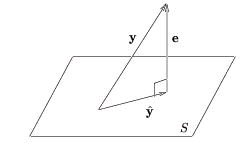
the subspace defined by the set {x∈ V|(x ⊥ S)} . When S is closed, we can write V=( S⊕ S⊥) The orthogonal projection of y onto S, where S is a closed subspace of V, is
s.t.
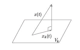
is an ON basis for S. Orthogonal projection yields the best approximation of y in S:
The approximation error
obeys the orthogonality principle:
(e ⊥ S) We illustrate this concept using V=ℝ3 (Figure 4.10) but stress that the same geometrical interpretation applies to any Hilbert space.
Figure 4.10.


A proof of the orthogonality principle is:
()
4.3. Discrete Wavelet Transform
Discrete Wavelet Transform: Main Concepts*
Main Concepts
The discrete wavelet transform (DWT) is a representation of a signal x( t)∈ ℒ 2 using an
orthonormal basis consisting of a countably-infinite set of wavelets. Denoting the wavelet basis as
, the DWT transform pair is
()
()
where { d k , n } are the wavelet coefficients. Note the relationship to Fourier series and to the
sampling theorem: in both cases we can perfectly describe a continuous-time signal x( t) using a
countably-infinite ( i.e. , discrete) set of coefficients. Specifically, Fourier series enabled us to
describe periodic signals using Fourier coefficients { X[ k]| k∈ℤ} , while the sampling theorem
enabled us to describe bandlimited signals using signal samples { x[ n]| n∈ℤ} . In both cases,
signals within a limited class are represented using a coefficient set with a single countable index.
The DWT can describe any signal in ℒ 2 using a coefficient set parameterized by two countable
indices:
.
Wavelets are orthonormal functions in ℒ 2 obtained by shifting and stretching a mother wavelet,
ψ( t)∈ ℒ 2 . For example,


()
defines a family of wavelets
related by power-of-two stretches. As k increases,
the wavelet stretches by a factor of two; as n increases, the wavelet shifts right.
When ∥ ψ( t)∥=1 , the normalization ensures that ∥ ψ k , n ( t)∥=1 for all k∈ℤ , n∈ℤ .
Power-of-two stretching is a convenient, though somewhat arbitrary, choice. In our treatment of
the discrete wavelet transform, however, we will focus on this choice. Even with power-of two
stretches, there are various possibilities for ψ( t) , each giving a different flavor of DWT.
Wavelets are constructed so that
( i.e. , the set of all shifted wavelets at fixed scale k),
describes a particular level of 'detail' in the signal. As k becomes smaller ( i.e. , closer to –∞ ), the
wavelets become more "fine grained" and the level of detail increases. In this way, the DWT can
give a multi-resolution description of a signal, very useful in analyzing "real-world" signals.
Essentially, the DWT gives us a discrete multi-resolution description of a continuous-time
signal in ℒ 2 .
In the modules that follow, these DWT concepts will be developed "from scratch" using Hilbert
space principles. To aid the development, we make use of the so-called scaling function
φ( t)∈ ℒ 2 , which will be used to approximate the signal up to a particular level of detail. Like
with wavelets, a family of scaling functions can be constructed via shifts and power-of-two
stretches
()
given mother scaling function φ( t) . The relationships between wavelets and scaling functions will
be elaborated upon later via theory and example.
The inner-product expression for d k , n , Equation is written for the general complex-valued case. In our treatment of the discrete wavelet transform, however, we will assume real-valued
signals and wavelets. For this reason, we omit the complex conjugations in the remainder of
our DWT discussions
The Haar System as an Example of DWT*


The Haar basis is perhaps the simplest example of a DWT basis, and we will frequently refer to it
in our DWT development. Keep in mind, however, that the Haar basis is only an example; there
are many other ways of constructing a DWT decomposition.
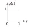
For the Haar case, the mother scaling function is defined by Equation and Figure 4.11.
()
Figure 4.11.
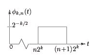
From the mother scaling function, we define a family of shifted and stretched scaling functions
{ φ k , n ( t)} according to Equation and Figure 4.12
()
Figure 4.12.
which are illustrated in Figure 4.13 for various k and n. Equation makes clear the principle that incrementing n by one shifts the pulse one place to the right. Observe from Figure 4.13 that is orthonormal for each k ( i.e. , along each row of figures).
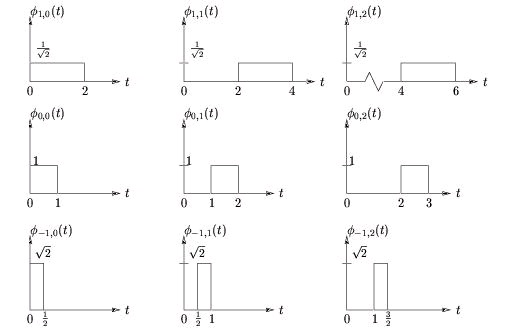


Figure 4.13.
A Hierarchy of Detail in the Haar System*
Given a mother scaling function φ( t)∈ ℒ 2 — the choice of which will be discussed later — let us
construct scaling functions at "coarseness-level-k" and "shift- n" as follows:
Let
us then use Vk to denote the subspace defined by linear combinations of scaling functions at the
k th level:
In the Haar system, for example, V 0 and V 1 consist of signals with
the characteristics of x 0( t) and x 1( t) illustrated in Figure 4.14.
Figure 4.14.
We will be careful to choose a scaling function φ( t) which ensures that the following nesting
property is satisfied: …⊂ V 2⊂ V 1⊂ V 0⊂ V-1⊂ V-2⊂ … coarse detailed In other words, any signal in Vk can be constructed as a linear combination of more detailed signals in V k − 1 . (The Haar
system gives proof that at least one such φ( t) exists.)
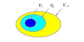


The nesting property can be depicted using the set-theoretic diagram, Figure 4.15, where V − 1 is represented by the contents of the largest egg (which includes the smaller two eggs), V 0 is
represented by the contents of the medium-sized egg (which includes the smallest egg),
Describe what you're looking for in as much detail as you'd like.
Our AI reads your request and finds the best matching books for you.
Popular searches:
Join 2 million readers and get unlimited free ebooks